
What Is Sensitivity Analysis?
Sensitivity analysis is the study of how uncertainty in a model output (or response) can be attributed to different sources of uncertainty in the model inputs (or factors). These analyses are powerful tools for modeling and simulation activities, as they allow the modeler to identify the most and least influential parameters on the key predicted outputs of interest. Not only does knowing the important parameters allow the modeler to focus on a select few inputs for design work, but perhaps more importantly, identifying the negligible parameters allows a modeler to omit them from difficult optimization problems by setting them to constant values, thereby simplifying the optimization task.
The data science literature contains several sensitivity analysis methods. A general characteristic among them is a trade-off between number of required model evaluations and amount of information that can be extracted. For example, the so-called Sobol method can quantify the first-order, second-order, and even factor-factor interaction effects on a response of interest, but it often requires multiple thousands of model evaluations to extract this type of detailed information. As a result, we usually only perform the Sobol method on fast-executing metamodels.
The Elementary Effects Method
In contrast, this study focuses on the Elementary Effects method (sometimes called the Method of Morris), which has an advantage of being computationally efficient by requiring a relatively low number of model evaluations. However, the outputs of the method are not as detailed. As a result, it is good at providing a general ranking of many parameters, and for this reason it is particularly useful for identifying parameters with negligible influence that can be discarded from subsequent optimization or Design of Experiments studies.
For example, this method was successfully applied to over 40 parameters of a GT-SUITE engine friction model to reduce the complexity of an optimization, as described in this paper: https://www.jstor.org/stable/26926852. This blog will similarly apply the method to a battery model prior to an optimization task.
The Elementary Effects Method is best explained by considering a simple system of 2 inputs (factors) and 1 output (response). The XY plot below has the two factors on the two axes so that the entire domain (defined by the range of each factor) can be visualized (here the two factors are given equal and arbitrary ranges of 0 to 10).
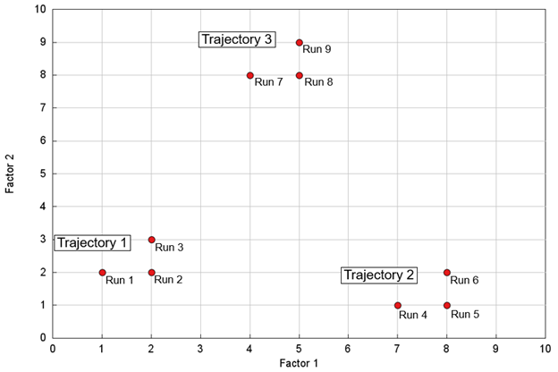
The method uses one-at-a-time sampling to change a single factor at a time between each model evaluation (simulation). The sampling method works as follows:
- The first model evaluation (run 1) is randomly chosen within the domain, where this example uses factor values of (1, 2).
- Run 2 occurs after making a step change to factor 1, where the step change in this example is 1.
- Run 3 occurs after keeping factor 1 constant and making a step change to factor 2.
- After completing these first 3 model evaluations, we can now calculate an elementary effect, EE, for each factor, where an EE is the linear change in response (R) with respect to the factor change. The subscript indicates the run number.
Factor 1 EE=|(R² -R¹)/(F² - F¹ )| Factor 2 EE=|(R³ -R²)/(F³ - F² )|
- The set of F+1 runs (where F is the number of factors) is called a trajectory, and the above process is repeated for k total trajectories, where each trajectory begins in a different, randomly chosen location in the domain. The plot above shows 3 example trajectories, but the total number is often in the range of 15-30, where a smaller number might be more appropriate for a smaller number of factors, and vice versa for a larger k.
- After performing all the runs, k different elementary effects are obtained for each factor. The distribution of these different EEs informs us about the sensitivity of each factor on the response. Specifically, the average and standard deviation of each factor’s set of EEs is calculated, then compared to those of the other factors.
The sensitivity analysis results are conveniently summarized in a single plot for each response, where each factor appears as a single point on the plot, with the x-axis representing the mean of the EEs, and the y-axis representing the standard deviation. Factors whose points lie near the origin have little or negligible effect on the response. Factors whose points lie far from the origin have the most influence on the response. The values are standardized and normalized so that the axes span 0 to 1, and a threshold of 0.1 is commonly used to identify negligible factors.
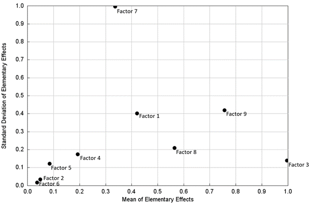
The above plot shows:
- Factors 3, 7, and 9 have the largest influence on the response.
- Since large means indicate large first-order effects, factors 3, 9, 8, and 1 have the largest first-order effects on the response, in that order.
- A large standard deviation indicates either a large higher-order effect or a large interaction effect with one or multiple other factors. Unfortunately this method cannot distinguish between the two, nor can it identify the other factor(s) that might be interacting. Although factor 7 only has a low-to-moderate first-order effect, it has a large standard deviation, making it important.
- Factors 2, 5, and 6 have means and standard deviations that lie below the commonly used threshold of 0.1, which means they can confidently be labeled as negligible or having low influence.
Although the Elementary Effects method has limitations in the level of information it can provide, it adequately provides a ranking of factors, and perhaps more importantly, it is computationally efficient in requiring a relatively low number of model runs equal to k(F+1). As an example, a system with 9 parameters might only need (15 trajectories)(9+1) = 150 model evaluations for sufficient analysis. In comparison, a common method to quantify first-order effects is to perform linear least-squares analysis using a 2-level full-factorial Design of Experiments, which would entail 29 = 512 model runs. The Elementary Effects method could be applied to a model having 34 parameters with only (25 trajectories)(34+1) = 875 model runs, whereas a 2-level full-factorial would require an impractical 234 = 1.7E10 model runs.
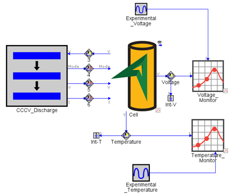
The Battery Model
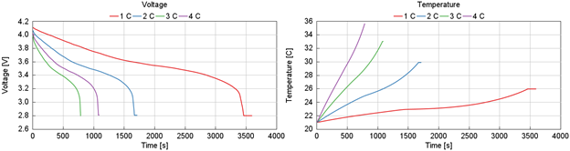
The GT-SUITE battery model used in this study is a 1D AutoLion battery model configured to characterize the voltage and temperature responses at 4 different constant current operating conditions.
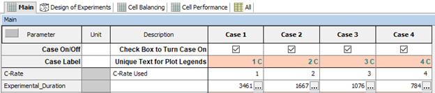
Case Setup consists of 4 cases of increasing C-Rates.
The main model results of interest are the transient cell voltage decrease and cell temperature increase. The plots below show the experimental data to which the model would eventually be calibrated. The purpose of the sensitivity analysis is to identify which parameters to use in the optimization.
More information on the calibration process for electrochemical battery models can be found with in this blog.
Sensitivity Analysis on the Battery Model
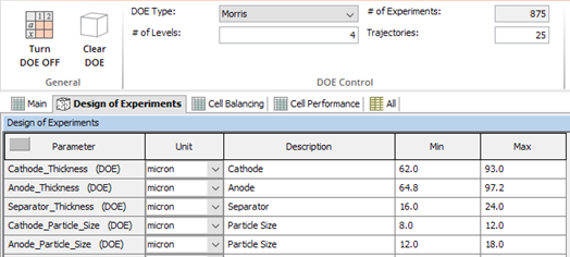
The Elementary Effects method is applied in GT-SUITE using a Design of Experiments. The battery parameters are added to the Design of Experiments folder in Case Setup, and the “Morris” DOE type is selected, and lower and upper limits are entered for each parameter. The “# of Levels” field determines the grid from which samples can be randomly chosen; the first plot in this blog illustrated 10 levels, but 4 levels is more commonly used. 25 trajectories are used, resulting in 875 experiments per case. The screenshot below shows only the first 5 parameters.
It is probably unnecessary to perform the analysis on all 4 C-Rate cases, so to save computation time, only the lowest and highest C-Rate cases will be run. As a result, a total of 1750 simulations will be run.
The sensitivity analysis results will be automatically provided in the DOE post-processor, but because this tool only works with scalar data and not transient profiles, each voltage and temperature profile must be reduced to a single numeric value. Integrators will be used for that purpose – “Int-V” and “Int-T” parts can be seen on the map layout above. The integrated quantities will serve as the responses for the analysis.
After running the 1750 simulations, the .glx result file is opened in GT-POST. A button in the Home tab provides quick access to the DOE post-processor, and the sensitivity analysis results are available in the Analyze Experiments page of the post-processor. The plots summarizing the EEs for all factors are provided below.
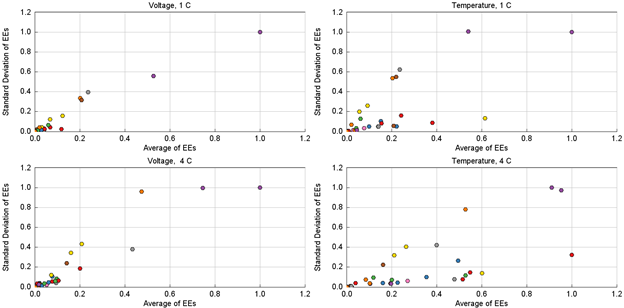

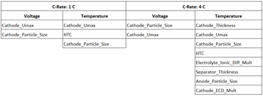
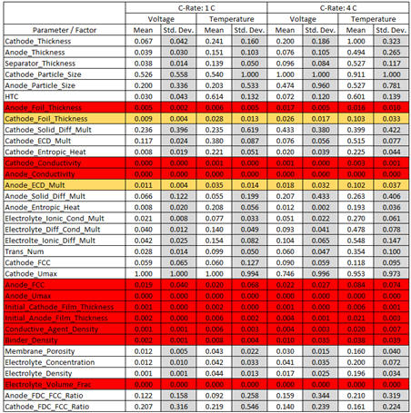
Screenshots of the plots are not as helpful as interacting with them in the post-processor, so the results are also provided in the following tables. The first table ranks the most influential parameters on each output variable, in order of main effect (average of elementary effects), among those that are above 0.5. Cathode_Umax and Cathode_Particle_Size have significant effects on both the voltage and temperature and at both C-Rates. The second table provides a full tabulation of the sensitivity analysis results. The 10 parameters that have mean and standard deviations less than 0.1 for both voltage and temperature, and for both C-Rates, are highlighted red, indicating they can be confidently removed from subsequent optimization or DOE studies. Two parameters have a single value that is slightly above the 0.1 threshold and are highlighted yellow, so these could also be omitted from subsequent studies.
Why The Elementary Effects Method Is Useful
The Elementary Effects method is a useful modeling tool to gain insights to how a large number of parameters are affecting a model. As a computationally efficient method for sensitivity analysis that requires a relatively low number of model evaluations, it can rank all the parameters, identify the most important ones, and identify the negligible ones. Applying the Elementary Effects method to a battery model having 34 parameters prior to optimization resulted in identifying 10 or 12 parameters that had negligible impact on the voltage and temperature results of interest. As a result, the optimization problem’s complexity could be reduced by working with 22 or 24 parameters, instead of 34.